Simulations with PICwriter
The 3-dimensional geometry of all PICwriter components (a scalar dielectric function) can be exported to an HDF5 file format for simulation using various open-source and commercial electromagnetic simulation software. Convenient functions are also provided for automatically computing the transmission/reflection spectra of PICwriter components with arbitrary numbers of ports (specified by their portlist) using freely available finite-difference time-domain (FDTD) software (MEEP). The pymeep python package must be installed to use the functions available below.
In order to specify the vertical profile in the vertical (out-of-plane) direction, the user must first specify a `MaterialStack` object that is responsible for mapping each mask layer/datatype to a vertical stack of materials.
Defining 3D geometries using PICwriter
The mapping of GDSII layers/datatypes to vertical dielectric profiles is done by creating a MaterialStack object and adding VStacks for each layer/datatype to be considered. An example of creating a MaterialStack is given below:
import picwriter.picsim as ps

epsSiO2 = 1.444**2
epsSi = 3.55**2
etch_stack = [(epsSiO2, 1.89), (epsSi, 0.07), (epsSiO2, 2.04)]
mstack = ps.MaterialStack(vsize=4.0, default_stack=etch_stack, name="Si waveguide")
waveguide_stack = [(epsSiO2, 1.89), (epsSi, 0.22), (epsSiO2, 1.89)]
clad_stack = [(epsSiO2, 1.89), (epsSi, 0.05), (epsSiO2, 2.06)]
mstack.addVStack(layer=1, datatype=0, stack=waveguide_stack)
mstack.addVStack(layer=2, datatype=0, stack=clad_stack)
First, we import the picsim library. Next, we specified the dielectric constant for the two materials considered (silicon and silicon dioxide at a wavelength of 1550 nm). Then, we create a VStack list (etch_stack), that is in the format [(dielectric1, thickness1), (dielectric2, thickness2), …]. With this we can create the MaterialStack object, with etch_stack the default vertical stack in the domain. Next, we create a waveguide_stack VStack list and associate it with the (1,0) GDSII layer using the addVStack call.
Quickly computing mode profiles
With a properly defined material stack, PICsim makes it easy to quickly view the mode profile corresponding to your layout’s WaveguideTemplate with the compute_mode() function:
import picwriter.components as pc
wgt = pc.WaveguideTemplate(bend_radius=15, wg_width=0.5, clad_width=3.0,
wg_layer=1, wg_datatype=0, clad_layer=2, clad_datatype=0)
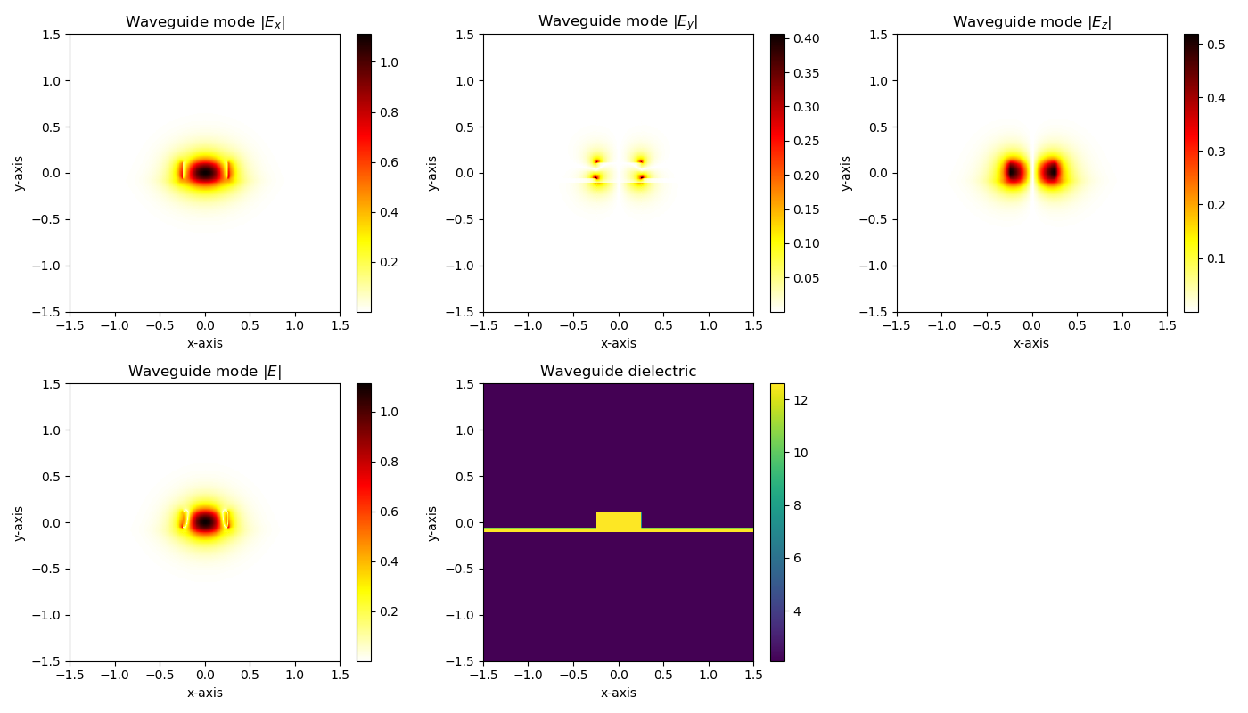
ps.compute_mode(wgt, mstack, res=128, wavelength=1.55, sx=3.0, sy=3.0,
plot_mode_number=1, polarization="TE")
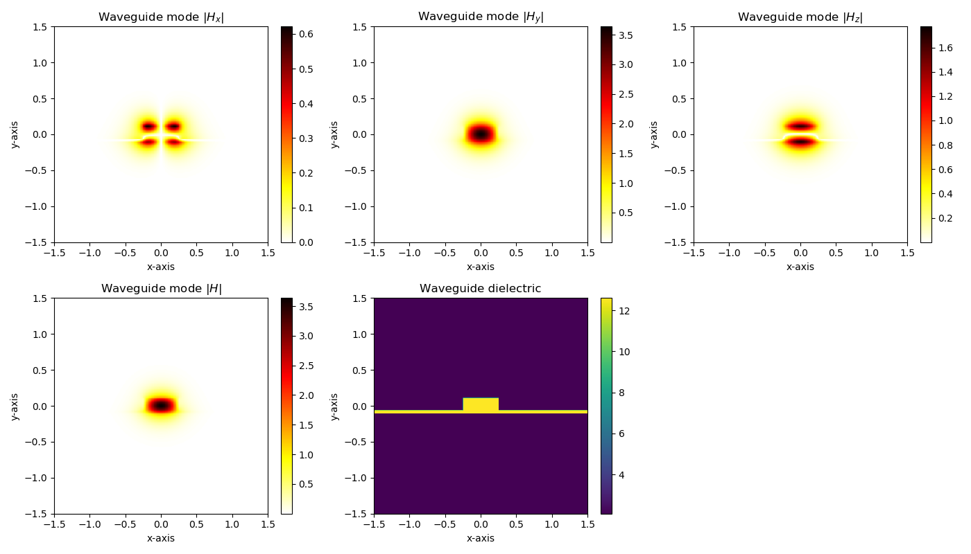
Which produces plots of the corresponding electric fields:
and magnetic fields:
Computing the transmission/reflection spectra
Likewise, we can build a PICwriter component in the normal way and directly launch a MEEP simulation. Below we build a DirectionalCoupler object and give it 2 um of waveguide at all the inputs/outputs (this will be useful when we simulate with MEEP later):
import picwriter.toolkit as tk
from picwriter.components import *
import numpy as np
import gdspy

top = gdspy.Cell("top")
wgt = WaveguideTemplate(bend_radius=15, wg_width=0.5, clad_width=3.0,
                        wg_layer=1, wg_datatype=0, clad_layer=2, clad_datatype=0)

simulated_component = gdspy.Cell('sc')

dc = DirectionalCoupler(wgt, 3.5, 0.2, angle=np.pi/16.0,
                                            parity=1, direction='EAST', port=(0,0))
tk.add(simulated_component, dc)

x0,y0 = dc.portlist['input_top']['port']
x1,y1 = dc.portlist['input_bot']['port']
x2,y2 = dc.portlist['output_top']['port']
x3,y3 = dc.portlist['output_bot']['port']

PML_wg1 = Waveguide([(x0,y0), (x0-2,y0)], wgt)
PML_wg2 = Waveguide([(x1,y1), (x1-2,y1)], wgt)
PML_wg3 = Waveguide([(x2,y2), (x2+2,y2)], wgt)
PML_wg4 = Waveguide([(x3,y3), (x3+2,y3)], wgt)

tk.add(simulated_component, PML_wg1)
tk.add(simulated_component, PML_wg2)
tk.add(simulated_component, PML_wg3)
tk.add(simulated_component, PML_wg4)
The gdspy Cell object simulated_component now contains four short waveguides and a DirectionalCoupler object. In order to launch a MEEP simulation and compute transmission/reflection spectra, we need to tell PICwriter what ports we want to monitor the flux through:
ports = [dc.portlist['input_top'],
         dc.portlist['input_bot'],
         dc.portlist['output_top'],
         dc.portlist['output_bot']]
The first port specified in the list above will be the inport where MEEP will place an EigenmodeSource. The last step is calling compute_transmission_spectra with the simulated component, MaterialStack, ports, and some additional information about the simulation:
ps.compute_transmission_spectra(simulated_component, mstack, wgt, ports, port_vcenter=0,
                            port_height=1.5*0.22, port_width=1.5*wgt.wg_width, dpml=0.5,
                            res=20, wl_center=1.55, wl_span=0.6, fields=True,
                            norm=True, parallel=False)
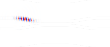
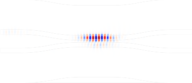
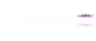
In the above port_vcenter specifies the center of the port in the vertical direction, port_height and port_width are the cross-sectional size of the power flux planes, res is the resolution (in pixels/um), wl_center and wl_span specify the center wavelength and wavelength span of the input pulse (in um), fields = True tells MEEP to output images of the electric field profile every few timesteps, norm = True tells MEEP to first perform a normalization calculation (straight waveguide) using the wgt WaveguideTemplate parameters. parallel specifies if the simulation should be run using multiple processor cores (requires MEEP/MPB to be built using parallel libaries), and n_p then specifies the number of cores to run on.
NOTE: This function requires MEEP and MPB to be compiled (from source) together, so that MEEP can call MPB to input an EigenmodeSource at the first port location.
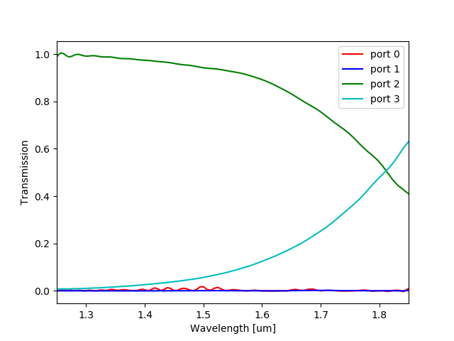
The resulting structure that is simulated and several field images are shown below:
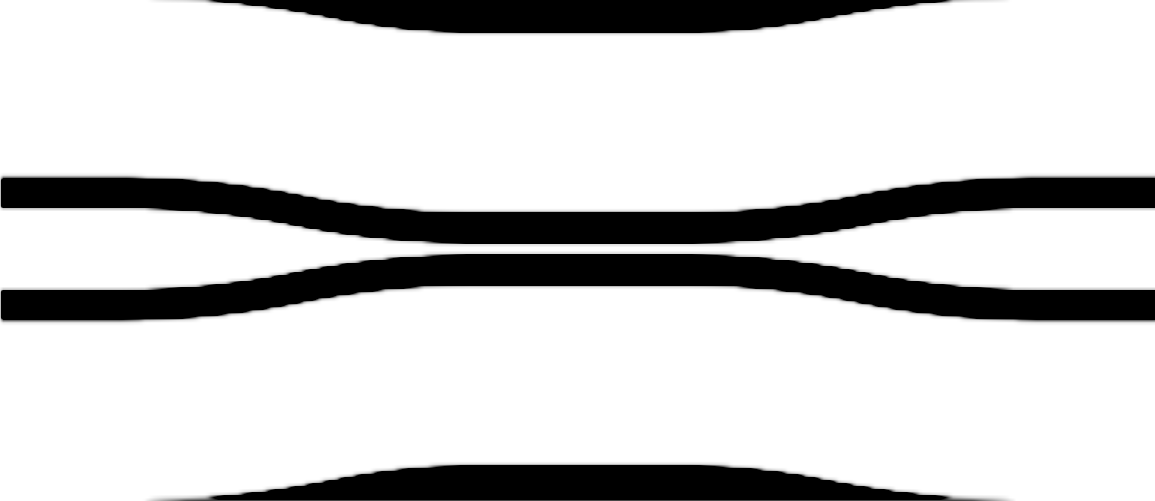
The compute_transmission_spectra() function will also compute and plot the appropriately normalized transmission/reflection spectra, saving the .png image in the working directory. The raw power flux data is also saved in .out and .dat files in the working directory.